7. Conditional formatting
Conditional formatting allows you to define a formatting (essentially font or background colors of cells, etc.) that will be applied to cells meeting a condition. This has the advantage of highlighting cells that meet certain criteria or showing variations or trends.
A great advantage with this technique is that after defining conditional formatting, Excel automatically updates the formatting, every time you make updates at your sheet.
To define conditional formatting, we will use:
- Either the Conditional Formatting command from the Home tab of the ribbon
- Or the Quick Analysis button
We are going to give you an overview of this Quick Analysis button. Next, we will see a multitude of real-life examples of conditional formatting.
7.1. The Quick Analysis button
This button, introduced from the 2013 version of Excel, appears as soon as you select a range of cells ... at the lower right corner of the selection: ![]()
Click on the Quick Analysis button, to see conditional formatting options.
|
If the selected cells contain only text, the options that appear are:
|
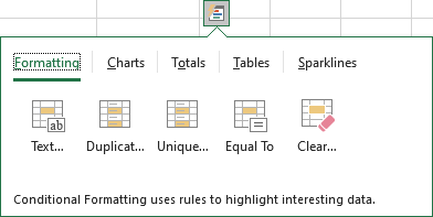 |
|
If the selected cells contain numbers, the options that appear are:
|
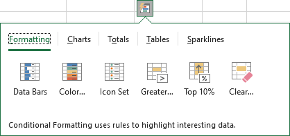 |
Other conditional formatting commands are available from the Conditional Formatting command in the Styles group on the Home tab of the ribbon.
7.2. Values less than, greater than, between
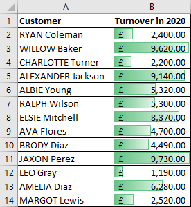
Consider the following excerpt from a spreadsheet:
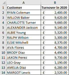
Let's apply some formatting for the values in column B as follows:
- Values greater than 8000 in green
- Values between 4000 and 8000 in yellow
- Values less than 4000 in red
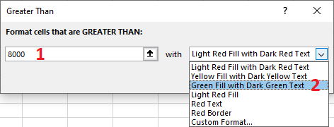
Select the range B2:B14 and click on the Conditional Formatting command on the Home tab of the ribbon, choose Highlight Cells Rules, then choose Greater Than:
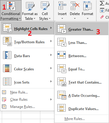
In the Greater Than dialog box that appears, enter the value 8000 and select Green Fill with Dark Green Text:
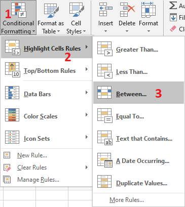
Keep the range B2:B14 selected and click the Conditional Formatting command on the Home tab of the ribbon, choose Highlight Cells Rules, then choose Between:
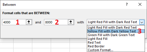
In the Between dialog box, enter the value 4000, the value 8000 and select Yellow Fill with Dark Yellow Text:
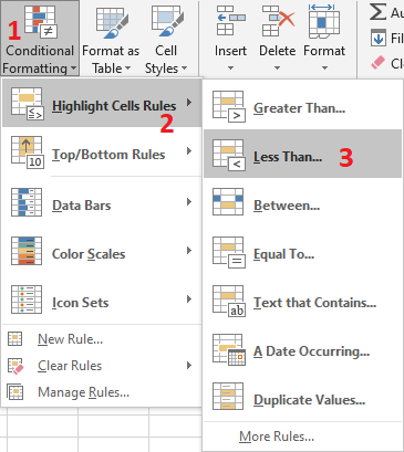
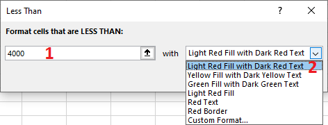
Select the range B2: B14 again and click the Conditional Formatting command on the Home tab of the ribbon, choose Highlight Cells Rules, then choose Less Than:
In the Less Than dialog box, enter the value 4000 and select Light Red Fill with Dark Red Text:
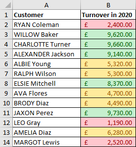
Here is the result:
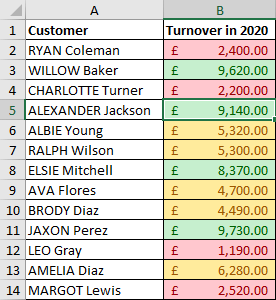
Modify a value; for example, at line 4, put the value 2200 and validate with the Enter key on the keyboard. Notice that cell B4 automatically turns red:
7.3. Cells containing text
Consider the following spreadsheet extract:
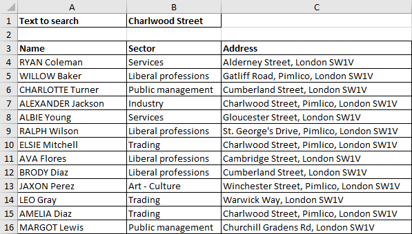
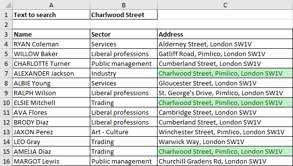
Suppose we want to show the inhabitant cases at Charlwood Street. Let's do the following:
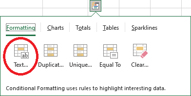
Select the range C4:C16. The Quick Analysis button ![]() appears at the bottom of the selection. Click on the Quick Analysis button then on the button Text That Contains:
appears at the bottom of the selection. Click on the Quick Analysis button then on the button Text That Contains:
The Text That Contains dialog box appears:
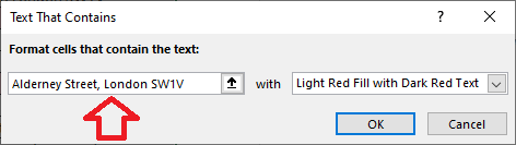
At this dialog, you can enter the text sought, that is to say, "Charlwood Street." But, since the searched text is written in cell B1, click on that cell. Excel adds the value "=$B$1". The advantage is that, if you want to search for another text, you just have to type it in cell B1, without having to redo the formatting.
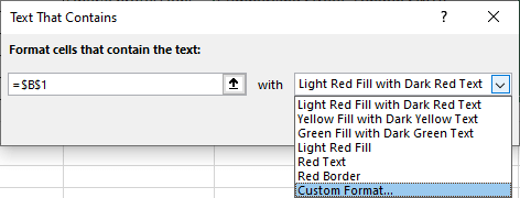
In the list of formats, you can choose a format from the list or choose Custom Format…
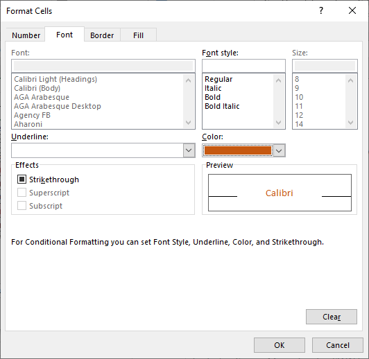
By choosing Custom Format…, the Format Cells dialog box appears. You can compose here the format that suits you by using the 4 tabs of this dialog box:
Choose a format and validate by clicking on the OK button.
Then click on the OK button in the Text That Contains dialog box. Notice the fields highlighted using the format you chose:
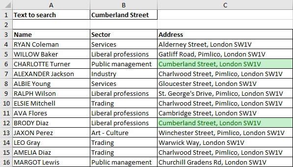
Now, modify the text of cell B1 by "Cumberland Street" for example, and validate with the Enter key on the keyboard. Notice that the formatting is updated automatically by Excel:
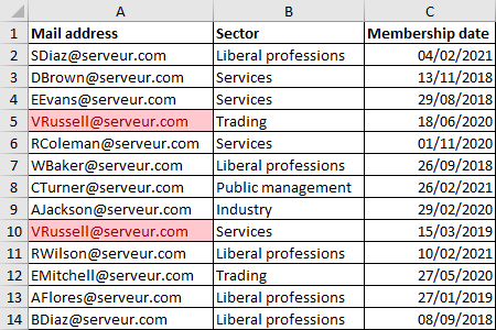
7.4. Duplicate values
Let's take the extract of the following spreadsheet containing in column A Mail addresses:
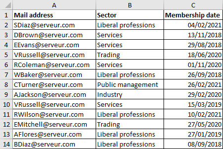
Normally, there should not be any duplicate email addresses, otherwise it is a typing error. So let's use this conditional formatting technique to find and correct any duplicates.
Select the range A2:A14 and click on the Quick Analysis button and then on the Duplicate Values button:
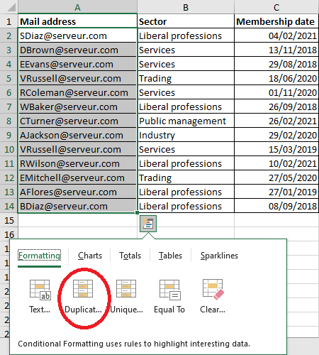
Excel highlights duplicate values in the selection:
7.5. Data Bars
Consider the following extract from a spreadsheet:
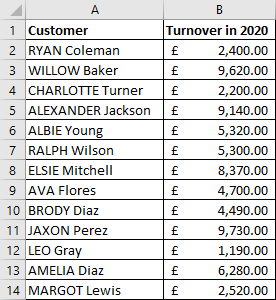
Select the range B2:B14 and click on the Quick Analysis button and then on the Data Bars button:
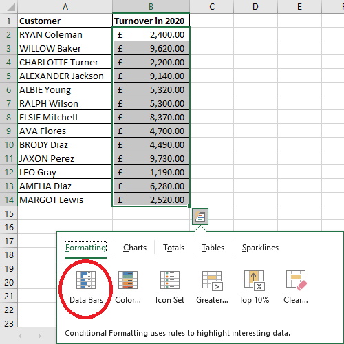
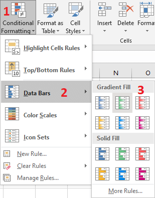
You can do this in a different way. Select the range B2:B14 and click on the Conditional Formatting command on the Home tab of the Ribbon, choose Data Bars, and then choose the colour you want:
Excel shows the importance of the values in the selection in a similar way to a graph:
7.6. Icon Sets
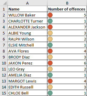
Consider the following extract from a spreadsheet:
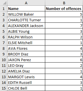
Select the range B2:B15 and click the Conditional Formatting command on the Home tab of the Ribbon, choose Icon Sets, then choose an icon set:
![]()
The result is as follows:
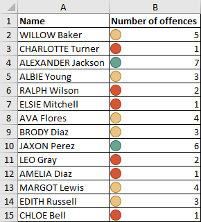
The disadvantage with this result is that the green colour indicates large numbers of offences (6 and 7), whereas it should indicate small numbers. On the other hand, I suppose we want a different distribution between the 3 colours, e.g:
- Red colour for 4 and more
- Orange colour for 2 and 3
- Green colour for 1
To get this result, proceed as follows:
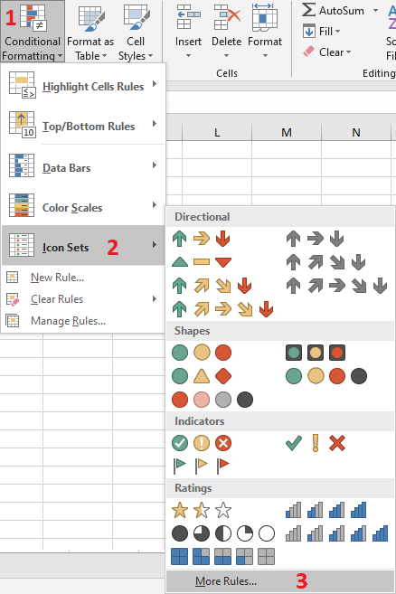
Select the range B2:B15 again and click on the Conditional Formatting command on the Home tab of the Ribbon, choose Icon Sets and then choose More Rules:
The New Formatting Rule dialog box appears:
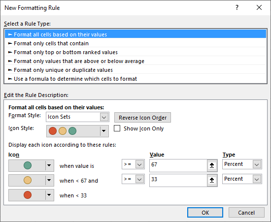
Click on the Reverse Icon Order button, change the Type to "Number" and the values as follows:
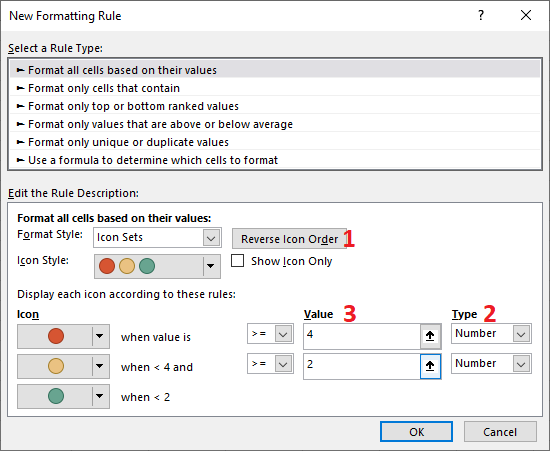
Confirm with the OK button. You should have the following result:
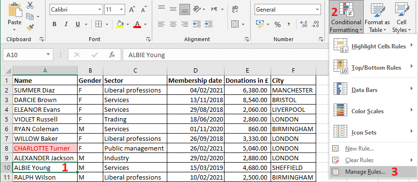
7.7. New formatting rule
Consider the following spreadsheet extract:
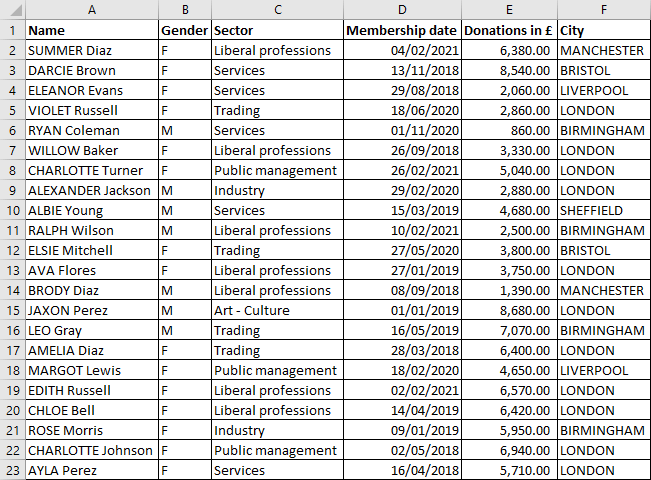
We want to highlight the names of subscribers whose donations exceed £4,000 and who live in London, for example. To do this, we will create a new formatting rule.
- Select the range of cells in column A where the names of the subscribers are written. For example the range A2:A80.
- Click on the Conditional Formatting command on the Home tab of the Ribbon, choose New Rule...
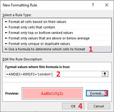
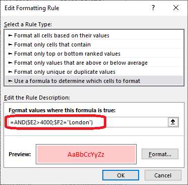
In the New Formatting Rule dialog box that appears :
- Click on Use a formula to determine which cells to format from the list Select a Rule Type...
- In the Format values where this formula is true field enter the formula :
=AND(E2>4000;F2="London")
The result of this formula is true when the conditions 'E2>4000' and 'F2="London"' are both true. See our sections on Excel 2016 Functions for more information on the AND function.
- Then click on the Format... button to open the Format Cells dialog box and choose the format that suits you. The use of this dialogue box is mentioned in section 7.3. above.
- Confirm with the OK button.
Here is the result:
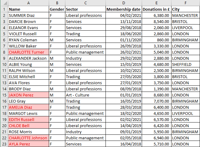
I would like to draw your attention to the fact that in the formula I have used the addresses of cells E2 and F2. These cells correspond to the first cell of the selection. That is to say, the one situated at the top left of the selection; that is to say, A2. The formula is applied to the other cells in the selection in a similar way to the Autofill.
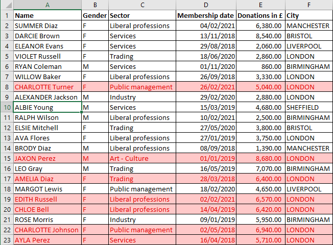
And if we want to highlight the whole row for which the condition is true. Like this:
Explanations in the next section.
7.8. Viewing and modifying formatting rules
Let's modify the rule defined in the previous section to highlight the whole row for which the condition is true:
- Click on a cell in the range A2:A80; where the conditional formatting is defined
- Click on the Conditional Formatting command on the Home tab of the Ribbon, choose Manage Rules...
- The Conditional Formatting Rule Manager dialog box opens:
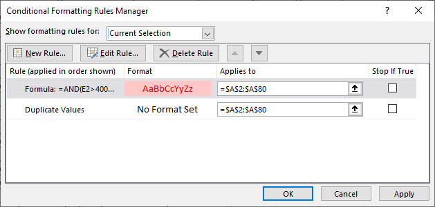
In this dialogue box,
- You can display the formatting rules for :
- The current selection
- The current sheet
- Or each sheet of the current workbook
- The list of rules is displayed in the table below. In the extract above, two rows corresponding to two formatting rules
- The buttons New Rule..., Edit Rule... and Delete Rule... allow you, as their names indicate, to
- Create a new formatting rule
- Modify the rule selected in the list below
- Delete the rule selected in the list below
I remind you that we want to modify the rule defined in the previous section in order to highlight the whole line for which the condition is true, i.e.; donations greater than 4000 and city equals London. To do this, in the Conditional Formatting Rules Manager dialog box:
- Edit the Applies to field for the rule to :
=$A$2:$F$80
NB. Note that this field is editable in the dialog box.
NB. You can now click on the OK button and see the result. The rest of the line does not take the defined formatting.
Why not? I remind you again that with the relative cell references E2 and F2, Excel increments the E and F for the cells in columns B, C, ... This means that for cell B2 for example, Excel will check the conditions in cells F2 and G2...
You must, therefore, change the formula of the rule to : =AND($E2>4000;$F2="London"). To do this:
- Click on the line of the rule we want to modify
- Click on the button Edit Rule...
- In the Edit Formatting Rule dialog box that appears, enter the following in the Format values where this formula is true field:
=AND($E2>4000;$F2="London")
- Click the OK button to return to the Conditional Formatting Rules Manager dialog box
- Click on the OK button and see the result:
7.9. Clear conditional formatting
To clear the conditional formatting for a range of cells, select that range of cells and use the Quick Analysis button, then the Clear Rules button:
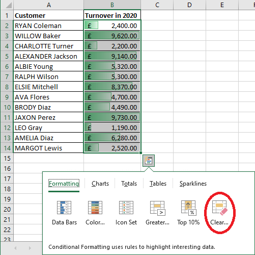
NB. You can undo a conditional formatting by going through the Conditional Formatting Rules Manager dialog box as mentioned in the previous section.
7.10. Copy of conditional formatting
| As this is a layout, copying it from one cell range to another must be done using the Format Painter button |  |
But, if you make a copy of cell contents, for example, using the Autofill technique, then the formatting is copied by Excel at the same time.