6. Use of calculations

---

6.1. Writing formulas

With Excel, you can do automatic calculations:

Enter in a cell "=8+4" and validate with the Enter key on the keyboard. You will of course have the value 12.

First, note that to enter a formula and ask Excel to calculate it, you must first write "=" followed by the formula and then confirm with the Enter key on the keyboard or with the Enter button on the Formula Bar.

 

I still specify, that if you do not start by writing "=", Excel will not make any calculation, and will always display "8+4".

6.2 Operands

The values 8 and 4 of the previous formula are called operands. The advantage is that we can use cells as operands. Here is an example :

• Enter for example 4 in cell A2 and 8 in cell A3
• In cell A4, enter "=A2+A3" and validate. Cell A4 will have the value 12.

At the formula level, we entered the addresses of cells "A2" and "A3". We can have them entered by Excel as follows:

• Click on cell A4
• Enter "=" using the keyboard
• Click with the mouse on cell A2
• Enter "+" using the keyboard
• Click on the cell A3 with the mouse
• Validate

A formula can also contain an operand which is itself a formula. Here is an example :

• Enter the value 5 in cell A5
• Enter in cell A6: "=A4*A5"
• Validate

Here we used cell A4 which itself contains a formula. Excel can handle complicated worksheets where cells are dependent on each other.

The advantage is that; if we modify the value in cell A2 for example with the value "6", cells A4 and A6 will automatically have the values 14 and 70 respectively without having to enter the formulas another time. Although Excel displays the result of the expression at the cell level, it still retains the formula you entered.
To review the formula used at the cell level, simply:

• Click on this cell
• See the formula in the formula bar.

NB. If you have an error or the result at the cell level does not suit you, you will need to review the formula giving that error. To do this, click on the corresponding cell to see the formula on the formula bar.

6.3 Operators

Arithmetic operators are the most used in Excel. There are 7 of them:

Arithmetic operator	Meaning	Example	Resault
+	Addition	5+2	7
-	Substraction Negation	5-2 -2	3 -2
*	Multiplication	5*2	10
/	Division	5/2	2.5
%	Percentage	20%	0.2
^	Power	5^2	25

There are also comparison operators. These operators combine two mainly numeric operands and result in a logical value; that is, TRUE or FALSE. I present to you the list of these operators, and I will show you their interests later using examples:

Comparison operator	Meaning	Example	Resault
=	Equal to	5=3	FALSE
>	Greater than	5>3	TRUE
<	Less than	5<3	FALSE
>=	Greater than or equal to	5>=3	TRUE
<=	Less than or equal to	5<=3	FALSE
<>	Different from	5<>3	TRUE

The text concatenation operator, with the symbol "&", allows to combine 2 texts to give a single one:

Text operator	Meaning	Example	Resault
&	Concatenation	"Hello" & "everybody"	Hello everybody

This is useful for example if we have a column with first names and another column with last names and we want to have a column with first names and last names.

Reference operators result in a reference to a range of cells:

Reference operators	Meaning	Example	Resault
:	Range operator	B5:B15	Cell range from B5 to B15
,	Union operator	B5:B15,D5:D15	Cell range from B5 to B15 and cells from D5 to D15
(space)	Intersection operator	B7:D7 C6:C8	Range of common cells between ranges B7:D7 and C6:C8

Operator priority order

Excel processes operations from left to right. However, there are operators who have priority over others. For example, multiplication takes precedence over addition. The formula "2+3*4" is equivalent to "2+(3*4)".

It is therefore necessary to know precisely this order of priority, otherwise use the parentheses to impose the order that suits you.

6.4 The SUM function

Excel has a multitude of functions that can be used in formulas. We will immediately show the example of the SUM function.

• Fill the cells in the range A2:A15 with numeric values
• In cell A16, enter "="
• Note that the Name Box no longer displays the address of the active cell, but the name of a function. Click the small arrow to the right to open a list of functions. Select the SUM function.
• The Function arguments dialog box is open. In this box, you will specify the range of cells to use for the calculation of the sum. Notice that Excel suggests the range A2:A15 to you. This is the case when adjacent cells are filled with numeric values.
• You can accept the proposed cell range and click on the OK button.
• Otherwise, enter a different range in the Number1 box or select the desired range using the mouse.

You can do it another way to get the same result:

• Fill the cells in the range A2:A15 with numeric values
• Select cell A16 and click on the SUM button in the Edit group of the Home tab of the ribbon . Make sure the range of cells offered is the one you want.
• Another method is to first select the range of cells A2:A15 and then click on the SUM button. In this case, the sum will be entered in the cell A16 just below.
• Validate with the Enter key or the Enter button in the formula bar.

 

6.5 Copying formulas

Once we have entered a formula in a cell, we can copy this formula to other cells, either using Copy/Paste, or using the technique Autofill that we saw in section 5.

• Reproduce the following example on an Excel sheet

 

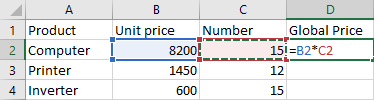
• In cell D2, enter the formula "=B2*C2". Confirm with the Enter key on the keyboard.
• Now click on cell D2 to select it.
• Position the mouse pointer at the right-bottom corner of cell D2, click and hold and drag to cell D4.

NB. You can also use the Copy/Paste buttons in the Clipboard group on the Home tab for the copy. This is useful for example, if you need to copy to a nonadjacent cell.

Note that the formula copied to cell D3, is "=B3*C3" and not "=B2*C2". That is to say that Excel adapts the references of the ranges when copying. This is what we want in this case and it is desirable in the majority of cases.

The adaptation of the cell plage references made by Excel during the copying is as follows:

• Excel increments all the line numbers of the cell references during a vertically incremented downward copy. This is the case for the references B2 and C2 incremented respectively in B3 and C3 then in B4 and C4
• Excel increments all the column numbers of the cell references during a horizontally incremented copy to the right. If I copy for example the formula "=B2*C2" horizontally to the right, I will have:
  • "=C2*D2" in cell E2
  • "=D2*E2" in cell F2

However, there are cases where this adaptation is not desirable. Take the following example:

 

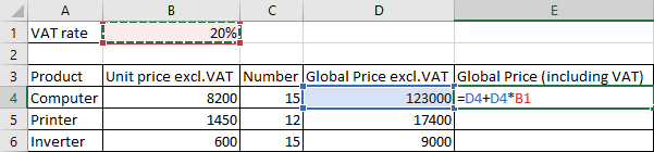
• At the cell E4, the formula is "=D4+D4*B1".
• If I recopy for cells E5 and E6, I will have the formulas "=D5+D5*B2" and "=D6+D6*B3" respectively. Now, what we want is that B1 is used constantly in the 3 formulas.
• This is possible by writing the address of cell B1 in the formula as "$B$1". Enter the following formula in cell E4: "=D4+D4*$B$1" and validate.
• Now do the copying for cells E5 and E6 and notice.

The form $B$1 is called an absolute cell reference. The form B1 is called the relative cell reference.

NB. You can switch from the absolute cell reference to the relative cell reference and vice-versa either by adding or removing "$" or by clicking on the "F4" key on the keyboard.

Finally, I point out that we may need the absolute reference to be only relative to the column or only relative to the row. For example, for the above case, it is sufficient to use the form B$1. As, we copied vertically, the B is not likely to change and we do not need to fix it.

For the case of the following multiplication table, find the right formula to put in cell B2 and have it copied throughout the rest of the table?

 

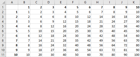
Use the formula "=$A2*B$1" in cell B2, copy to cell B11 and then copy to column K.

Exercises

Exercise 1 – Calculation, Formulas and Series

Exercise 2 – Calculation, Formulas and Series

Exercise 3 – Calculation, Formulas and Series

Exercise 4 – Calculation, Formulas and Series

---