3. Manipulation of cell ranges

---

In Excel, we often talk about range of cells. It’s just part of a spreadsheet. Whether it is a cell or several, continuous or not. it can also be one or more columns or rows.

3.1. Selection of cell ranges

Selecting a range of cells means making it active. You should know how to make cell range selections. The reason is that in order to apply a command to a range of cells, you must first select it. In other words, when you click a button, the underlying command is applied to the selected range.

3.1.1. Selection of continuous cell range

To select a range of continuous cells:

• Click and hold the mouse pointer over a cell at an end of the range. The pointer should be like this:
• Move the pointer to the cell at the other end of the range then release the mouse pointer

Another method which is particularly useful when the cell range is very large:

• Click on a cell at an end of the range
• Click and hold the Shift button on the keyboard
• Click on the cell at the other end of the range and release the Shift button

3.1.2. Selection of columns or rows

To select a column or a row click on its header. The mouse pointer when clicking must be of this shape  to select a column and of this shape  to select a row.

To select several columns or several rows:

• Click without releasing the mouse pointer on the header of the first row or column of the target range
• Move the pointer to the header of the last row or column of the target range
• Now release the mouse pointer

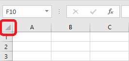
3.1.3. Selection of the whole sheet

To select the entire worksheet, use the Select all button:

3.1.4. Selecting ranges of discontinuous cells

To select ranges of discontinuous cells, follow these steps:

• Select a first continuous range
• Hold down the Ctrl key
• Select the other ranges

3.2. Moving cell ranges

You can move the contents of a range of cells to another location in your spreadsheet. For that :

Select the range of cells you want to move Move the mouse pointer to the edge of the range until the pointer becomes this shape When the pointer is of the aforementioned shape, click without releasing Move the pointer to the place you want, then release.

NB. You can also duplicate the contents of the cell range, for this, proceed as for the movement by holding down the Ctrl key on the keyboard during the movement.

3.3. Inserting rows or columns

To insert a row to a worksheet

• Select a cell above which the row will be added
• Use the Insert command in the Cells group of the Home tab and choose Insert Sheet Rows.

NB. To insert several lines at once:

• Select a range of cells with as many rows as you want to add. That is, if you want to insert 4 rows for example, just select 4 cells vertically.
• Use the Insert command in the Cells group of the Home tab and choose Insert Sheet Rows.

To insert a column to a worksheet:

• Select a cell to the left of which the column will be added
• Use the Insert command in the Cells group of the Home tab and choose Insert Sheet Columns.

NB. To insert several columns at the same time:

• Select a range of cells that have as many columns as you want to add. That is, if you want to insert 4 columns for example, just select 4 cells horizontally.
• Use the Insert command in the Cells group of the Home tab and choose Insert Sheet Columns.

3.4. Insert blank cells with shift cells right or down

To insert empty cells with cells shift left or down:

• Select the range of cells where you want to insert the blank cells
• Use the Insert command in the Cells group of the Home tab and choose Insert Cells .... The Insert dialog box appears
• Choose Shift cells right or Shift cells down. And validate with the OK button.

3.5. Deleting a range of cells with shifting cells to the left or up

• Select the range of cells concerned
• Use the Delete command from the Cells group of the Home tab and choose Delete Cells .... The Delete dialog box appears.
• In the Delete dialog box, choose the option that suits you Shift cells left or Shift cells up. Then, validate using the OK button.

NB. If you use the Delete button of the keyboard, the contents of the range will be erased. But, there will be no cell shift.

3.6. Hide and unhide rows or columns

We can hide rows or columns without having to permanently delete them. This is useful for example if there are columns involved in calculations or filtering data and we don't want them to appear with the result.

I also point out that when printing a sheet, hidden columns and rows are not included in the print. We can therefore temporarily hide columns that we do not want to print.

To hide columns:

• Select one or more columns or just a range of cells from these columns.
• Use the Format command in the Cells group of the Home tab and choose Hide & Unhide then Hide Columns.

In the same way, to hide rows:

• Select one or more rows or just a range of cells from those rows.
• Use the Format command in the Cells group of the Home tab and choose Hide & Unhide then Hide Rows.

To display hidden columns:

• Make a selection including the hidden columns. For example, select a column to the right and one to the left of the hidden columns
• Use the Format command in the Cells group of the Home tab and choose Hide & Unhide then Unhide Columns.

To display hidden rows:

• Make a selection including the hidden rows. For example, select a row above and a row below the hidden rows
• Use the Format command in the Cells group of the Home tab and choose Hide & Unhide then Unhide Rows.

3.7. Freeze panes

We use this function in case we have a table with a large number of rows and we want to keep the row with the column headers always visible when we scroll down the page.

Suppose the column headers are on row 3 for example. We will therefore freeze rows 1 to 3 in this way:

• Select the cell A4
• On the View tab of the ribbon, use the Freeze Panes command in the Window group and choose Freeze Panes.

---